The most exciting feature of Apache Spark is it’s ‘generality’ meaning the ability to rapidly take some text data, transform it to a graph structure and perform some network analysis with GraphX take that dataset and apply some machine learning algorithms with SparkML and store it in memory and query it using SparkSQL all within a single program of very little code.
In this post I wanted to write about the Spark ML framework and how easy and effective it is to do scalable machine learning by creating a pipeline which perform Natural Language Processing to assess whether a user’s plain text review aligns with their rating (from 1 to 5).
The dataset I have chosen is an Amazon Reviews dataset which has been nicely curated by Julian McAuley from University of California, San Diego for use with their Machine Learning papers:
Image-based recommendations on styles and substitutes J. McAuley, C. Targett, J. Shi, A. van den Hengel SIGIR, 2015
Inferring networks of substitutable and complementary products J. McAuley, R. Pandey, J. Leskovec Knowledge Discovery and Data Mining, 2015
1. Know your data
The first thing to note is that the authors, who have extracted the data using Python, have generated in a non-standard JSON format which means that Spark’s internal reader will not be able to read it. This tutorial was written with Spark 1.5.2 and from reading the Spark JIRA it looks like 1.6.0 will allow the Spark JSON reader to deal with non-standard JSON. Otherwise it can be fixed quickly and easily using the simple Python script the authors provide on their site:
import json
import gzip

def parse(path):
  g = gzip.open(path, 'r')
  for l in g:
    yield json.dumps(eval(l))

f = open("output.strict", 'w')
for l in parse("reviews_Video_Games.json.gz"):
  f.write(l + '\n')
I also took the opportunity to recompress the gzipped files to BZ2 so they would be splittable and could be more easily consumed downstream.
Let’s look at the first row in the reviews_Books.json.gz file as we will be using this dataset for the rest of this post:
{
  "summary": "Show me the money!",
  "overall": 4.0,
  "reviewerID": "AH2L9G3DQHHAJ",
  "unixReviewTime": 1019865600,
  "reviewText": "Interesting Grisham tale of a lawyer that takes millions of dollars from his firm after faking his own death. Grisham usually is able to hook his readers early and ,in this case, doesn't play his hand to soon. The usually reliable Frank Mueller makes this story even an even better bet on Audiobook.",
  "asin": "0000000116",
  "helpful": [5, 5],
  "reviewTime": "04 27, 2002",
  "reviewerName": "chris"
}
From this review we have learnt:
- There are two elements which we want for this tutorial. The
reviewTextwhich we need to parse and theoverallwhich tells us what score the customer actually rated the product. - Based on my mental model I wouldn’t be able to translate the
summary‘Show me the money!’ text to any useful rating so it is unlikely to help in translating the dataset. - In this review I can determine there are 53 words which is actually lower than Amazon’s recommended ‘ideal length …[of] 75 to 500 words’
- If we are getting
reviewTextwith as few as 53 words and potentially as much as 500+ word the model will have to be tuned to work out which words are important not just how frequently they appear. - As we know the
reviewerIDperhaps a model could incorporate some sort of adjustment factor for different reviewers that have skewed review scores compared to the population? - Perhaps the
helpfulratings could be used to add additional weighting to reviews by indicating that people who thought the review was helpful had semi-validated that the text aligned with the score.
In this exercise we are only going to use the reviewText and overall fields but potentially a much stronger model could be built with additional features.
The question is, can our model determine enough from the review text to accurately classify the text into one of the discrete 1.0, 2.0, 3.0, 4.0, 5.0 categories?
2. Load the Files
Copy reviews_Books.json.bz2 to somewhere on your filesystem that can be accessed by your Apache Spark process. For development we are going to execute these Scala scripts using the bin/spark-shell utility:
bin/spark-shell -i filename.scala
2.1 Setting up
Let’s start by loading libraries. You can see that this tutorial depends heavily on many different aspects of the spark.ml library particularly on the feature library which will do much of the data pre-processing for us:
import org.apache.spark.ml.Pipeline
import org.apache.spark.ml.PipelineModel
import org.apache.spark.ml.classification.NaiveBayes
import org.apache.spark.ml.classification.NaiveBayesModel
import org.apache.spark.ml.feature.{RegexTokenizer,StopWordsRemover,PorterStemmer,NGram,,HashingTF,VectorAssembler,StringIndexer,IndexToString}
import org.apache.spark.ml.tuning.{ParamGridBuilder, CrossValidator}
import org.apache.spark.ml.evaluation.MulticlassClassificationEvaluator
import org.apache.spark.mllib.util.MLUtils

import org.apache.spark.sql.Row
import org.apache.spark.sql.DataFrame
import org.apache.spark.storage.StorageLevel
2.2 Load and Parse the Data
Now to load the data is extremely easy as we are using dataframes which will happily consume JSON files and create an SQL queryable dataset:
val reviews = "data/reviews_Books.json.bz2"
var reviewsDF = sqlContext.read.json(reviews)
reviewsDF.registerTempTable("reviews")
Three lines! Thanks Spark.
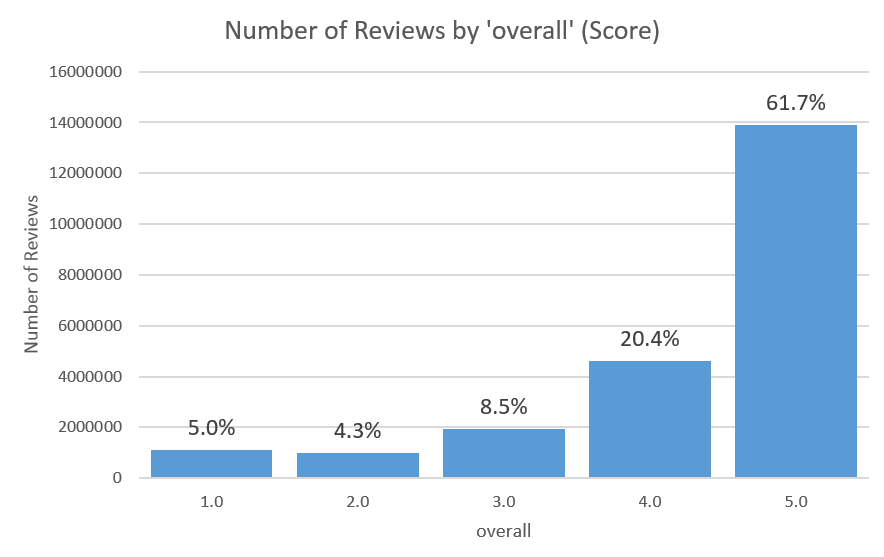
Now if we want to see the distribution of the 22507538 reviews we can run a very simple command. You can see that the data is massively skewed towards 5.0 star reviews (there are 14 5.0 reviews to every 1 2.0 review!
reviewsDF.groupBy("overall").count().orderBy("overall").show()

+-------+--------+
|overall|   count|
+-------+--------+
|    1.0| 1116877|
|    2.0|  978575|
|    3.0| 1922423|
|    4.0| 4602643|
|    5.0|13887020|
+-------+--------+
2.3 Prepare the data
I want to prepare a subset of my reviews dataset which meets two goals:
- Extract the same number of reviews from each
1.0,2.0,3.0,4.0,5.0category to train a generic model and ensure there are actually reviews for the model to learn from. - Separate
trainingandtestdata into two different datasets so that when we test the model it can in no way be influenced by thetrainingdata.
Why do I want the same number of reviews for each category? Skewed data, or having more training examples for one category than another, can cause the decision boundary weights to be biased. This causes the classifier to unwittingly prefer one class over the other. There is very good information available here about these biases.
In practice this means that the easy way of sampling data in Spark will, with this data set, produce a model which will appear to be performing classification very well but is in fact using a model which is highly skewed towards the 5.0 category:
reviewsDF = reviewsDF.sample(withReplacement = false,0.2)
To produce an equally weighted dataset we will use a SQL query because it makes it to easy to assign row numbers and choose an equal sized dataset for each category. I am ordering by rand() to take a quasi-random sample so if the model we build in this process is good I expect to get a very similar result every time we run this application on a different random dataset.
var reviewsDF = sqlContext.sql(
"""
  SELECT text, label, rowNumber FROM (
    SELECT
       reviews.overall AS label
      ,reviews.reviewText AS text
      ,row_number() OVER (PARTITION BY overall ORDER BY rand()) AS rowNumber
    FROM reviews
  ) reviews
  WHERE rowNumber <= 200000
  """
)

reviewsDF.persist(org.apache.spark.storage.StorageLevel.MEMORY_AND_DISK)

reviewsDF.groupBy("label").count().orderBy("label").show()
If we execute this code on a review dataset with at least 20000 reviews per category we would expect to see this result:
+-----+-----+
|label|count|
+-----+-----+
|  1.0|20000|
|  2.0|20000|
|  3.0|20000|
|  4.0|20000|
|  5.0|20000|
+-----+-----+
This dataset now has 100000 records containing a random set of reviews in each category which all have a rowNumber field from 1 to 20000 which means we can now easily split out a training and test dataset which is guaranteed to have the correct number of rows and be as random as Spark SQL’s rand() function is.
val training = reviewsDF.filter(reviewsDF("rowNumber") <= 15000).select("text","label")
val test = reviewsDF.filter(reviewsDF("rowNumber") > 15000).select("text","label")

training.persist(org.apache.spark.storage.StorageLevel.MEMORY_AND_DISK)
test.persist(org.apache.spark.storage.StorageLevel.MEMORY_AND_DISK)

val numTraining = training.count()
val numTest = test.count()

println(s"numTraining = $numTraining, numTest = $numTest")
3. Build the Pipeline
What is a pipeline anyway? Basically it is a series of steps (called stages) that are applied to a dataset in series which will transform the data.
3.1 A visual pipeline
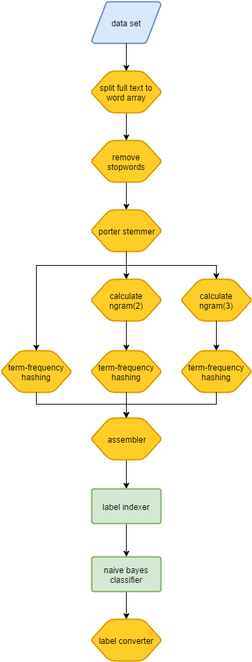
Let’s have a look at the pipeline we are building first so we can understand what is happening. You can see that the pipeline consists of:
- the blue box represents the data set as it is the input to the model. For the training stage of the model building we will pass the input data set as
trainingand when testing the model the data set will betest. - each of the yellow boxes represents a
transformstage which will take an input column from thetrainingdataset, perform some work and write out to an additional column in the dataset. Atransformerwill only operate on the current record. - the green boxes represent
estimatorsteps (such as theNaiveBayes()machine learning algorithm) which will process the entire dataset and produce model which can then be used totransforma subsequent dataset. Anestimatorwill operate over the entire dataset. - there are many more
transformsteps than anything else. This is because it is data and feature preparation which is the key work to prepare a machine learning model.
3.2 Now let’s code it
3.2.1 Split full text into array of words
First we need to process the raw text and convert it into an array of words. I found the RegexTokenizer is more useful than the default space-based (’ ‘) tokenizer as it will remove things like full stops and comma characters (.,,) and still deal with doesn't as a single token where \w would split it into doesn and t.
val regexTokenizer = { new RegexTokenizer()
  .setPattern("[a-zA-Z']+")
  .setGaps(false)
  .setInputCol("text")
}
Output:
Array([WrappedArray(interesting, grisham, tale, of, a, lawyer, that, takes, millions, of, dollars, from, his, firm, after, faking, his, own, death, grisham, usually, is, able, to, hook, his, readers, early, and, in, this, case, doesn't, play, his, hand, to, soon, the, usually, reliable, frank, mueller, makes, this, story, even, an, even, better, bet, on, audiobook)])
3.2.2 Remove Stopwords
The next step in text processing often involves removing low-information words such as ‘a’, ‘and’, ’the’. In the short review example above the word ‘his’ appears four times. Intuitively we can understand that this is not a particularly useful word for classification as it is not an emotive or descriptive word and it is likely to appear in many reviews for each category so it won’t help us split a positive from a negative review.
Because this function is so common it is built into the Spark core and you don’t even need to specify the list of words. If you are interested you can see the list in the source code or if you are very motivated you can provide your own list (maybe for some industries this would be beneficial). A quick way to generate stopwords is to run wordcount over a list of books and the most frequent n words are likely low information words or stopwords.
val remover = { new StopWordsRemover()
  .setInputCol(regexTokenizer.getOutputCol)
}
Output:
Array([WrappedArray(interesting, grisham, tale, lawyer, takes, millions, dollars, firm, faking, death, grisham, usually, able, hook, readers, early, case, doesn't, play, hand, soon, usually, reliable, frank, mueller, makes, story, better, bet, audiobook)])
3.2.3 Stemming
Stemming is a technique of reducing words to their root word or stem. For example, stems, stemmer, stemming, stemmed are all derivations of the root word stem. The reason we want to do this in a Natural Language Processor is to try to group words with the same meaning which should increase the frequency of that word occurring and hopefully it’s information value. Keep in mind that the stem word does not have be the correct morphological root, it just has to result in the same sequence of characters (in this algorithm play will stem to plai which doesn’t matter as long as played and playing also produces plai).
In the John Grisham example, an obvious stemming opportunity would be the first word, interesting which we can stem to interest. Theoretically if we found the word interested in another review we would also stem that to interest hopefully resulting in a stronger model.
As of Spark 1.5.2 Stemming has not been introduced but I have taken the Porter Stemmer Algorithm implemented in Scala by the ScalaNLP project and wrapped it as a Spark Transformer available here. Unfortunately, you are going to have to build Spark from source to use it.
val stemmer = { new PorterStemmer()
  .setInputCol(remover.getOutputCol)
}
Output:
Array([WrappedArray(interest, grisham, tale, lawyer, take, million, dollar, firm, fake, death, grisham, usual, abl, hook, reader, earli, case, doesn't, plai, hand, soon, usual, reliabl, frank, mueller, make, stori, better, bet, audiobook)])
3.2.4 Calculate n-grams
The most basic sentiment analysers use a list of words which have been loosely classified into positive (+1) and negative (-1) for each word:
good: 1
bad: -1
like: 1
hate: -1
The algorithm searches for those words in sentences and replaces then with a +1 or -1 score or 0 if not found (the mapper) and then sums up the resulting score (the reducer). But what happens when we give a more interesting sentence such as:
don't like
Depending on how basic the model is it is likely to come out as either positive (+1) due to the like (+1) keyword or maybe they also classify don't as a negative (-1) keyword which would sum to a 0 score. Either way, unless we consider both words as a pair we cannot interpret its true meaning and give the correct -1 score. Consider what would happen with a less abbreviated version such as ‘do not like’.
n-grams are a solution to this problem. A n-gram is a group of n words to be considered as a group. In the sentence above if we consider the ‘don’t like’ sentence as two words then a 2-gram algorithm world consider them as one feature. Then if we had a simple model and we set:
good: 1
bad: -1
don't like: -1
We can now calculate the correct sentiment score of -1.
In the workflow contained here we take the output of the PorterStemmer() stage and calculate n-grams of both 2 words and 3 words in length.
n-gram(2):
val ngram2 = { new NGram()
  .setInputCol(stemmer.getOutputCol)
  .setN(2)
}
Ouput:
Array([WrappedArray(interest grisham, grisham tale, tale lawyer, lawyer take, take million, million dollar, dollar firm, firm fake, fake death, death grisham, grisham usual, usual abl, abl hook, hook reader, reader earli, earli case, case doesn't, doesn't plai, plai hand, hand soon, soon usual, usual reliabl, reliabl frank, frank mueller, mueller make, make stori, stori better, better bet, bet audiobook)])
n-gram(3):
val ngram3 = { new NGram()
  .setInputCol(stemmer.getOutputCol)
  .setN(3)
}
Output:
Array([WrappedArray(interest grisham tale, grisham tale lawyer, tale lawyer take, lawyer take million, take million dollar, million dollar firm, dollar firm fake, firm fake death, fake death grisham, death grisham usual, grisham usual abl, usual abl hook, abl hook reader, hook reader earli, reader earli case, earli case doesn't, case doesn't plai, doesn't plai hand, plai hand soon, hand soon usual, soon usual reliabl, usual reliabl frank, reliabl frank mueller, frank mueller make, mueller make stori, make stori better, stori better bet, better bet audiobook)])
3.2.5 Term Frequency Hashing
At it’s core, a machine learning classifier is the process of determining the probability of a certain feature appearing in a certain class thereby allowing us to predict a likely classification based on an input containing one or more of those features.
If we had infinite compute then it would make sense to treat each distinct word or n-gram as a feature and calculate each one’s unique probability giving the most accurate model. The Oxford Dictionary has around 171,476 words in current use, and 47,156 obsolete words which is English only before all the spelling mistakes and abbreviations that are commonly found in Amazon reviews (go and try to read some smartphone game reviews if you want to know grammatical pain) so the problem space gets very large. Even having scalable architecture such as Spark does not forgive inefficient code.
Term Frequency Hashing helps as it is a dimensionality reduction technique to reduce the number of features by applying a hashing function. A key argument of the hashing function is how many discrete values or features will be produced and have their frequencies counted.
For example (and don’t do this) if we were to run a the Term Frequency Hashing transformer hashingTF() over the stemmed dataset with a target of two features by calling .setNumFeatures(2) we would get this result:
Array([WrappedArray(interest, grisham, tale, lawyer, take, million, dollar, firm, fake, death, grisham, usual, abl, hook, reader, earli, case, doesn't, plai, hand, soon, usual, reliabl, frank, mueller, make, stori, better, bet, audiobook)])

Array([(2,[0,1],[16.0,14.0])])
This means that the hashingTF() transformer has correctly produced two values (0,1) which have a count of 16 and 14 values respectively. The issue is that we have lost so much information by specifying so few features that the output is not useful for model building (we have deliberately created hash collisions due to such a small number of hash values).
If we run the same hashingTF() with 1000 features (.setNumFeatures(1000)) then we will see an array produced like this where the first line represents the hashed index value (which must be between 0 and 999) and the frequency. If you read the stemmed dataset you can see two words grisham and usually which appear twice and must have hashed to index of 583 or 589 in the hashing table (1000) as those are the only two which have frequency of 2.0. We don’t actually need to know which value is which as long as we use the same hashing function when we want to execute this model. The reason the dataset is so sparse is that we have only processed one row of data which has not produced 1000 distinct hash values from the words contained in that row.
Array([(1000,[15,50,128,170,187,192,204,207,210,230,236,266,354,371,422,425,483,508,519,575,583,589,600,624,698,908,991,997],[1.0,1.0,1.0,1.0,1.0,1.0,1.0,1.0,1.0,1.0,1.0,1.0,1.0,1.0,1.0,1.0,1.0,1.0,1.0,2.0,2.0,1.0,1.0,1.0,1.0,1.0,1.0,1.0])])
I want to apply the hashingTF() transformer against all my three working datasets but not specifying the number of features yet:
val removerHashingTF = { new HashingTF()
  .setInputCol(stemmer.getOutputCol)
}
val ngram2HashingTF = { new HashingTF()
  .setInputCol(ngram2.getOutputCol)
}
val ngram3HashingTF = { new HashingTF()
  .setInputCol(ngram3.getOutputCol)
}
3.2.6 Vector Assembler
After executing Term-Frequency Mapping across our three datasets we will end up with three vector columns containing hash indices and their term frequencies. VectorAssembler() will combine these columns into one so that it can be processed as the input column for the NaiveBayes algorithm we are going to run.
You can see from the Input/Output below that it will basically do a union of the datasets but will adjust the keys by the length of the hash function (1000) to avoid collisions. It is easy to see how this works by looking at the output at keys 991 and 1109. Because we know the HashingTF() function was set to product 1000 features the resulting indices can only be between 1 and 999. This means anything after 999 must be in the second set. As the value is 1109 and the first value in the second array is 109 you can see the transformer has added the length of the array (1000) to the key (109) and unioned the datasets.
Vector Assembler:
val assembler = { new VectorAssembler()
  .setInputCols(Array(removerHashingTF.getOutputCol, ngram2HashingTF.getOutputCol, ngram3HashingTF.getOutputCol))
}
Input:
Array([(1000,[50,170,187,192,204,230,266,317,355,363,391,422,425,428,467,474,483,492,519,575,600,602,611,854,908,972,981,991],[1.0,1.0,1.0,1.0,1.0,1.0,1.0,1.0,1.0,1.0,1.0,1.0,1.0,1.0,1.0,2.0,1.0,1.0,1.0,2.0,1.0,1.0,1.0,1.0,1.0,1.0,1.0,1.0])])
Array([(1000,[109,141,197,204,275,294,321,323,339,417,437,585,588,618,632,671,682,701,784,818,859,864,867,927,936,940,947],[1.0,1.0,1.0,1.0,1.0,2.0,2.0,1.0,1.0,1.0,1.0,1.0,1.0,1.0,1.0,1.0,1.0,1.0,1.0,1.0,1.0,1.0,1.0,1.0,1.0,1.0,1.0])])
Array([(1000,[10,87,92,101,178,180,278,312,329,368,384,431,473,522,523,589,677,695,718,729,742,811,877,879,936,957,971],[1.0,1.0,1.0,1.0,1.0,1.0,1.0,1.0,1.0,1.0,1.0,1.0,1.0,1.0,2.0,1.0,1.0,1.0,1.0,1.0,1.0,1.0,1.0,1.0,1.0,1.0,1.0])])
Output:
Array([(3000,[50,170,187,192,204,230,266,317,355,363,391,422,425,428,467,474,483,492,519,575,600,602,611,854,908,972,981,991,1109,1141,1197,1204,1275,1294,1321,1323,1339,1417,1437,1585,1588,1618,1632,1671,1682,1701,1784,1818,1859,1864,1867,1927,1936,1940,1947,2010,2087,2092,2101,2178,2180,2278,2312,2329,2368,2384,2431,2473,2522,2523,2589,2677,2695,2718,2729,2742,2811,2877,2879,2936,2957,2971],[1.0,1.0,1.0,1.0,1.0,1.0,1.0,1.0,1.0,1.0,1.0,1.0,1.0,1.0,1.0,2.0,1.0,1.0,1.0,2.0,1.0,1.0,1.0,1.0,1.0,1.0,1.0,1.0,1.0,1.0,1.0,1.0,1.0,2.0,2.0,1.0,1.0,1.0,1.0,1.0,1.0,1.0,1.0,1.0,1.0,1.0,1.0,1.0,1.0,1.0,1.0,1.0,1.0,1.0,1.0,1.0,1.0,1.0,1.0,1.0,1.0,1.0,1.0,1.0,1.0,1.0,1.0,1.0,1.0,2.0,1.0,1.0,1.0,1.0,1.0,1.0,1.0,1.0,1.0,1.0,1.0,1.0])])
3.3 Running the Model
At this point we have extracted all our features and at first I happily loaded them into the NaiveBayes() estimator, used it to transform my test dataset which produced nice 0.0,1.0,2.0,3.0,4.0 values which I then compared against my input labels which also look like 1.0,2.0,3.0,4.0,5.0 … with absolutely horrible results (~10%).

I was unlucky enough to have numeric labels as if I had strings such as (very good, good, …) it have highlighted the issue straight away: the NaiveBayes() transformer will produce indexed values as outputs. Using StringIndexer() means you should always ensure that predictions produced by the model can be mapped back to the original labels.
Fortunately it is very easy to convert to indexed values with StringIndexer() and back to their original labels with IndexToString().
3.3.1 Label Indexer
The StringIndexer() is actually an estimator which basically converts the distinct labels in the input dataset to index values e.g. (0.0,1.0,2.0,…n). The only trick it does is it will assign the indices in order of the frequency which the label appears in the dataset passed in the fit() parameter (and it has to assess the entire dataset to do so).
Label Indexer:
val labelIndexer = { new StringIndexer()
  .setInputCol("label")
  .setOutputCol("indexedLabel")
  .fit(reviewsDF)
}
Output:
// label, StringIndexer(label)
Array([4.0,0.0])
So when we have only one value we get label 4.0 = 0.0 but this automatic assigning of indexed values may trick you up unless you use the next transformer, IndexToString().
3.3.2 Label Converter
When the StringIndexer() it stores the mapping table allowing the IndexToString() transformer to convert indices back to the original label.
Label Converter:
val labelConverter = { new IndexToString()
  .setInputCol("prediction")
  .setOutputCol("predictedLabel")
  .setLabels(labelIndexer.labels)
}
Output:
// label, StringIndexer(label), IndexToString(StringIndexer(label))
Array([4.0,0.0,4.0])
Basically we just need to call that after our NaiveBayes() transformer to ensure our labels are correct.
3.3.3 Naive Bayes
I will leave WikiPedia to explain why Naive Bayes is a popular algorithm for Natural Language Processing tasks like spam filtering or sentiment analysis which is what we are doing here. Essentially it will calculate the probability of a certain word or phrase appearing for a given label and use that model to predict labels from new input data.
val nb = { new NaiveBayes()
  .setLabelCol(labelIndexer.getOutputCol)
  .setFeaturesCol(assembler.getOutputCol)
  .setPredictionCol("prediction")
  .setModelType("multinomial")
}